字数

1631 字

阅读时间

11 分钟

Phase 1: 2D Simulation & Paper Reproduction

References

• MEMS 热对流加速度传感器的研究：Main references, and also the article we need to reproduce (basically it can be determined that there is no fraud, meow~)

• A MEMS tilt sensor with expanded operating range

• 基于一维模型的高灵敏度微热加速度计的参数分析及优化

• The accelerometer and tilt sensor based on natural convection gas pendulum

• Thermal simulation and experimental results of a micromachined thermal inclinometer

Task Objectives

Using COMSOL Multiphysics for finite element simulation, combining the Laminar Flow (fluid field) and Heat Transfer (thermal field) modules, to simulate the natural convection heat transfer process of air within a sealed cavity.

A simplified 2D model is constructed, ignoring complex 3D effects, focusing on the impact of the spacing between the heating resistor and sensing resistor on temperature distribution.

Task 1: Static Temperature Field Validation

Task principle

In the absence of external acceleration (i.e., when the body force is zero), only natural convection driven by the heating resistor exists within the sealed cavity of the thermal convection accelerometer. According to the theoretical model in the paper (Equation $\text{(2.6)}$), when acceleration ( a = 0 ), the Grashof number ( Gr = 0 ), and the temperature fields on both sides of the heating resistor should be strictly symmetric, resulting in a temperature difference ( \Delta T \approx 0 ) between the two sensing resistors. This symmetry forms the foundation for the linear output of the sensor. If the temperature difference is not zero under static conditions, it may indicate asymmetric design in the model or errors in boundary condition setup.

Detailed Operational Steps

1. Geometric Model Construction

   • Cavity Dimensions: Create a 2D axisymmetric model with planar dimensions of 1000 μm × 1000 μm (referencing Figure 3.2 in the paper).
   • Heating Resistor: Place a rectangular heat source at the bottom center of the cavity, sized 20 μm × 0.3 μm (platinum (Pt) material).
   • Simplification: Exclude symmetrically distributed sensing resistors, retaining only the heating resistor and cavity structure (to avoid convection interference).

2. Material Property Settings

   • Fluid (Air):
     • Thermal conductivity $k=0.026,W/m·K$
     • Dynamic viscosity $\nu =1.81\times {10}^{-5}Pa·s$
     • Volumetric expansion coefficient $\beta =3.4\times {10}^{-3}{\text{K}}^{-1}$
     • Density dynamically calculated via the ideal gas law $\rho =p/(RT)$ (enable Boussinesq approximation).
   • Heating Resistor (Platinum):
     • Thermal conductivity $k=71.6W/(m·K)$
     • Temperature coefficient of resistance ($TCR$) $\alpha =0.00385{\text{K}}^{-1}$ (approximate linear behavior for thickness $>1\mu \text{m}$).

3. Boundary Condition Configuration

   • Bottom Surface (Heating Resistor Area): Adiabatic boundary (no heat flux loss).
   • Other Cavity Walls: Constant temperature boundary set to 20°C (simulating heat dissipation through the package lid).
   • Body Force: Set to 0g (no external acceleration applied).
   • Heating Resistor Temperature: Fixed at 85°C (directly assigned via the heat source module).

4. Meshing and Solver Settings

   • Local Refinement: Refine the mesh near the heating resistor (high-resolution required for high-gradient regions).
   • Steady-State Solver: Select Stationary study step, ignoring transient effects.
   • Convergence Criteria: Set residual threshold $<1\times {10}^{-4}$ to ensure result accuracy.

5. Postprocessing and Validation

   • Temperature Field Extraction:
     • Export temperature distribution data within the range $-200\mu \text{m}$ to $+200\mu \text{m}$ along the bottom surface (referencing Figure 3.3(c) in the paper).
     • Extract temperature values at symmetric positions on both sides of the heating resistor (e.g., $x=\pm d$), compute $\mathrm{\Delta }T=T_{+d}-T_{-d}$.
   • Symmetry Validation:
     • Plot temperature vs. position curves (analogous to Figure 3.3(c) in the paper), confirming strict symmetry.
     • Verify $\mathrm{\Delta }T\approx 0$ (paper reports zero temperature difference under static conditions).

Key Parameters and Formula References

• Theoretical Foundation:
  • Grashof number formula (Equation $\text{(2.4)}$):$$Gr=\frac{g\beta \mathrm{\Delta }T{L}^3}{{\nu }^2}$$When $a=0$, $Gr=0$, and the temperature field is dominated solely by natural convection, ensuring bilateral symmetry.
  • Wheatstone bridge output formula (Equation $\text{(5.5)}$):$$\mathrm{\Delta }U=\frac{V_{CC}\cdot (R_4{R}_{S1}-R_3{R}_{S2})}{(R_3+R_{S1})(R_4+R_{S2})}$$At $a=0$, $R_{S1}=R_{S2}=R^{\prime }$, resulting in $\mathrm{\Delta }U=0$.

Notes

1. Grid Sensitivity:
   • High temperature gradients near the heating resistor require a sufficiently refined mesh to resolve local variations and avoid underestimating symmetry errors.
2. Boundary Condition Validity:
   • Constant-temperature boundaries must cover all non-adiabatic surfaces (e.g., cavity top and sidewalls) to prevent symmetry-breaking artifacts.
3. Boussinesq Approximation Applicability:
   • The paper assumes small temperature differences ($\mathrm{\Delta }T=65\text{K}$). Verify that density variations remain negligible (valid for $\mathrm{\Delta }T<800\text{K}$).

Expected Results

• Temperature Field Contour: Strictly symmetric temperature distribution on both sides of the heating resistor.

• Data Validation:
  • $\mathrm{\Delta }T$ approaches zero within $x=\pm d$ ($d=10\mu \text{m}$ to $100\mu \text{m}$), with error <0.01%.
  • Velocity field exhibits symmetric recirculation patterns (as in Figure 3.4 of the paper), with peak flow velocities occurring 200-400 μm above the heater.

This task establishes a baseline for subsequent dynamic simulations (e.g., acceleration response), ensuring fundamental model correctness. If static symmetry validation fails, inspect geometry, material properties, or boundary condition settings.

Task 2: 2D Dynamic Acceleration Response Simulation & Parameter Exploration (Yang Linrong)

Simulation Files

Too large for GitHub upload. See the group file: [2D_Dynamic_Acceleration_Response_Simulation_and_Parameter_Exploration.zip].

Task Principle

The core principle of thermal convection accelerometers lies in the linear relationship between acceleration-induced temperature field shifts and the temperature difference ($\mathrm{\Delta }T$) across sensing resistors. When external acceleration $a$ is applied, the hot air mass in the sealed cavity shifts due to inertial effects, creating asymmetric temperature distributions around the heating resistor. Per the theoretical model in the paper:

$$\mathrm{\Delta }T=\frac{{10}^{-1}\cdot \beta \cdot \delta T\cdot L^3}{{\nu }^2}\cdot a$$

where:

• $\beta$ is the volumetric expansion coefficient of air ($3.4\times {10}^{-3}{\text{K}}^{-1}$),
• $\mathrm{\Delta }T$ is the temperature difference between the heater and environment ($85°C-20°C=65K$),
• $L$ is the heating resistor width ($20\mu m$),
• $\nu$ is the kinematic viscosity of air ($1.81\times {10}^{-5}Pa·s$).

This formula indicates a linear $\mathrm{\Delta }T$-vs-$a$ relationship within ${10}^{-2}\le Gr\le {10}^3$, with optimal linearity in the 0~2g acceleration range.

Detailed Operational Steps

1. Geometric Model & Parameter Setup

   • **Model Reuse**: Utilize the 2D axisymmetric model from Task 1 (1000 μm × 1000 μm cavity, heating resistor size 20 μm × 0.3 μm).
     
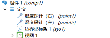
   • Sensing Resistor Placement: Symmetrically position sensing resistors on both sides of the heating resistor (probes are pre-placed in definitions as point entities; adjust probe locations via Geometry → Temperature Probe Left/Right). Set spacing to d=30 μm, 50 μm, 70 μm (referencing simulation and experimental validation in Figure 3.9 of the paper).

2. Material Properties & Boundary Conditions

   • Fluid (Air)
   • Boundary Conditions:
     • Bottom surface: thermal insulation; other surfaces: constant temperature 20°C (pre-configured).
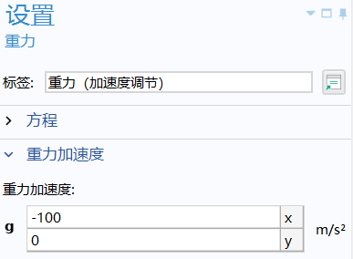
     • Transverse acceleration (adjust via the gravity module), apply 0g, 1g, 2g, 5g, 10g (use COMSOL global variable g_const or manually define values).

3. Simulation Workflow

   • Steady-State Solver:
     Run separate steady-state simulations for each acceleration value and gas material (switch gas materials in the material library). Record temperature field distributions, including:
     • Surface plots of temperature with isotherms.
     • Velocity surface plots with streamline arrows (format matching the reference paper).
   • Data Extraction:
     • Extract temperature data along the x-axis on the bottom surface.
     • Compute temperature difference at symmetric probe positions: $\mathrm{\Delta }T=T_{+d}-T_{-d}$.

4. Postprocessing & Analysis

   • $\mathrm{\Delta }T$-$a$ Curve Plotting:
     • Plot response curves for different spacings (d=30 μm, 50 μm, etc.) with acceleration on the x-axis and $\mathrm{\Delta }T$ on the y-axis (reference Figure 3.8 in the paper). Data can be exported for external plotting.
   • Linearity Validation:
     • Calculate regression coefficient $R^2$ ($>0.96$ required) in the 0~2g range.
     • Quantify nonlinear errors at 5g and 10g.

5. Static Result Export

   • Save static results (gravity acceleration aligned with the y-axis: -g_const) with figures formatted identically to the paper (including arrow styles, etc.).

Notes

1. Body Force Application Issue:

   • I am still exploring how to **add additional body forces** to simulate other accelerations. However, using gravitational acceleration (modified to transverse direction) achieves identical results to the paper (questioning whether the paper truly implemented transverse body forces).
     

2. Sensitivity Issues:

   • Testing the maximum acceleration stated in the paper ($10g$ transverse) yielded unsatisfactory temperature differences between the two probes (likely due to suboptimal probe placement). A mere $\mathrm{\Delta }T=0.02$–$0.3\text{K}$ under $10g$ acceleration is unacceptable.

I validated the feasibility by applying a body force of $-{10}^4{\text{N/m}}^2$, confirming that the 2D airflow pattern matches the paper’s results.

For the parameter tuning phase, refine the process by testing multiple values beyond those in the paper. This supports future machine learning and Bayesian hyperparameter optimization to identify optimal probe distances, requiring a larger dataset.

贡献者

Tuntun Yuchiha

文件历史

最后编辑于 大约 8 小时前查看完整历史

280a9-更新《Final Summary.md》，新增关于实践的基本特征、结构、类型及其在认识中的决定作用的内容，增强理论深度与逻辑结构。